はじめに
こんにちは。将棋と筋トレが好きな、情報系大学生のゆうき(@engieerblog_Yu)です。
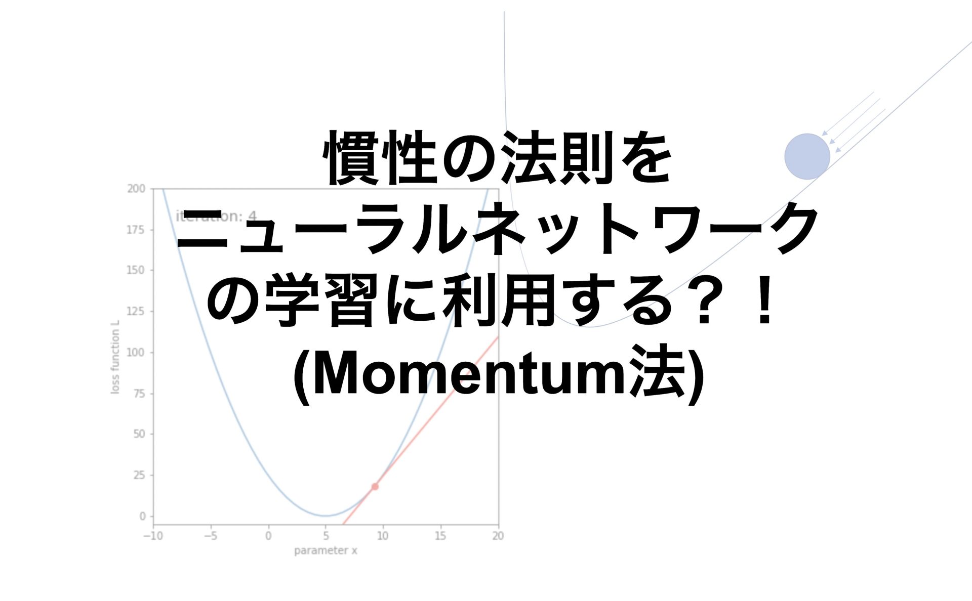
今回はニューラルネットワークの最適化問題を解く手法である、モーメンタム法についてまとめていきたいと思います。
Momentum法とは?
Momentum法は、勾配降下法に物理の慣性の法則を取り入れたようなものです。
Momentumとは「運動量」という意味を持っています。
Momentum法は以下の式で表されます。
\(v_{next} = αv_{initial} – η\frac{∂L}{∂x}\)
\(x_{next} = x_{initial} + v_{next}\)
前回の記事でも解説しましたが、勾配降下法は以下の式で表されます。
\(x_{next} = x_{initial} – η\frac{∂L}{∂x}\)
Momentum法は勾配降下法に速度を取り入れて、勾配方向に力を受けるという物理法則を表しています。
Momentum法のイメージ
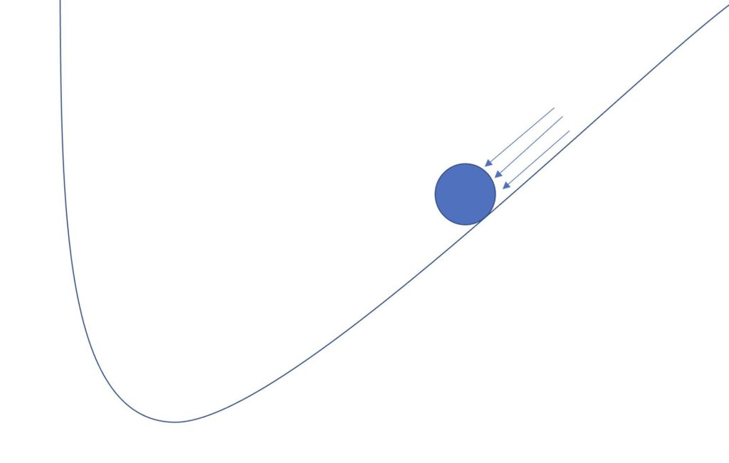
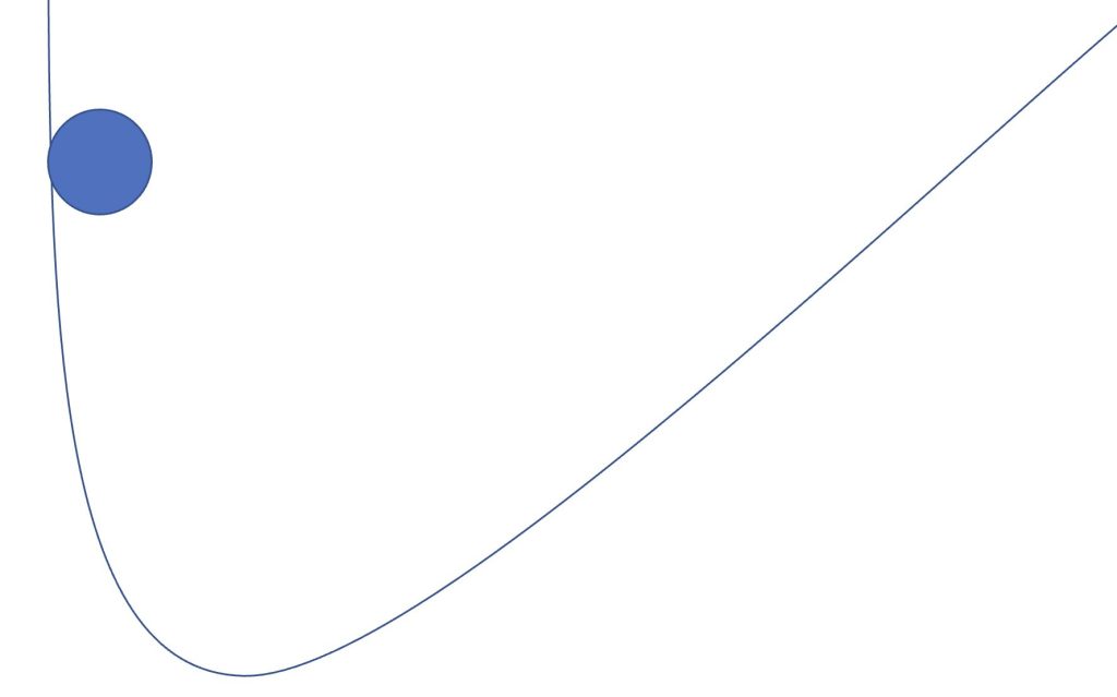
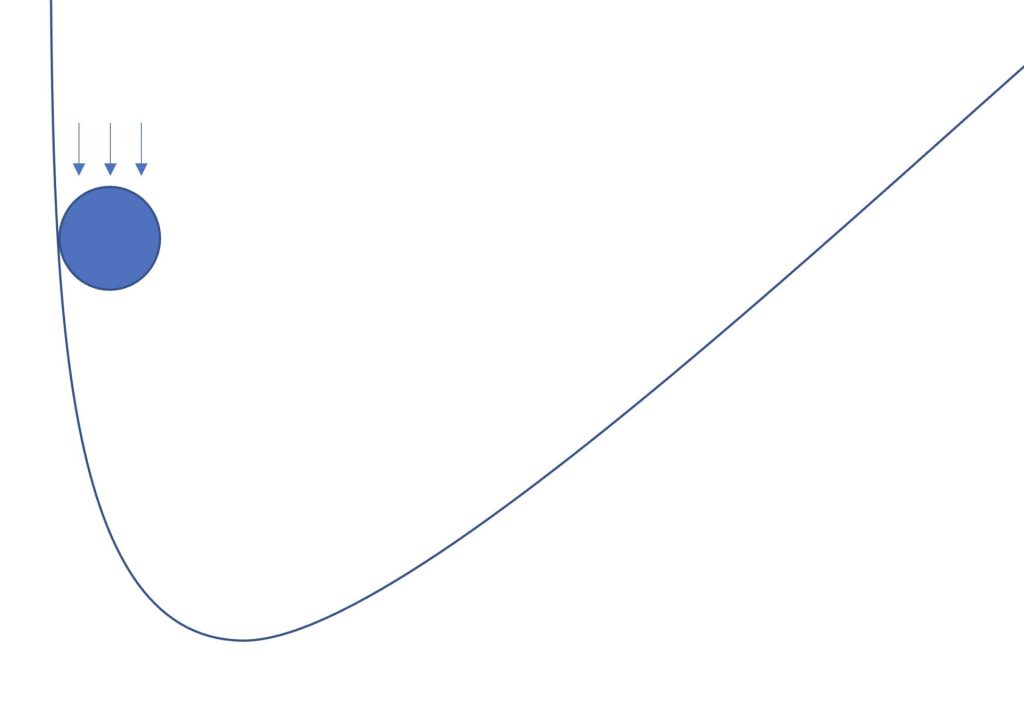
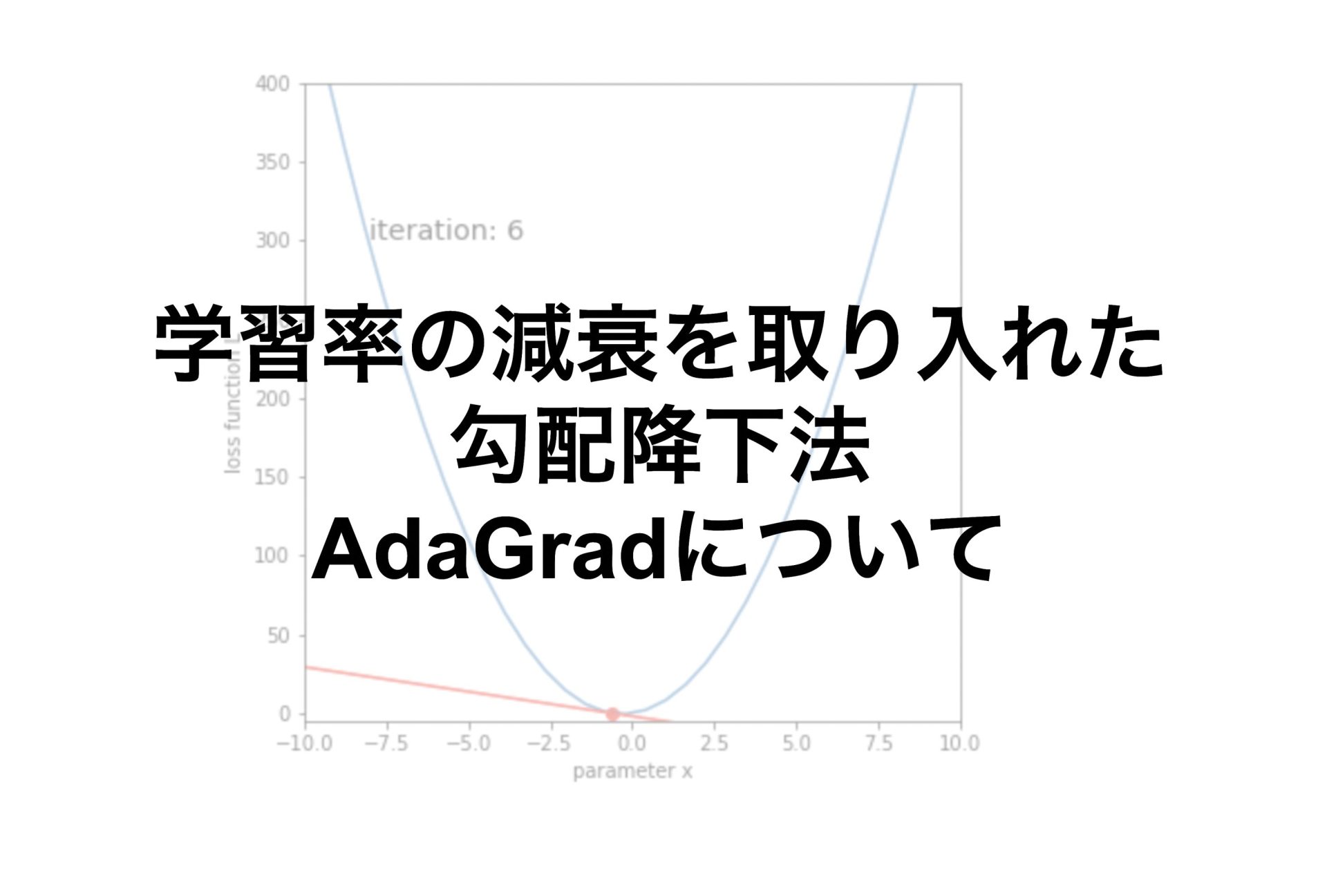
式では分かりにくいと思うので図で表すと以下のようになります。
Momentum法は、傾斜がある地面をボールが転がるような動きになります。
Momentum法の数式をもう一度記述します。
\(v_{next} = αv_{initial} – η\frac{∂L}{∂x}\)
\(x_{next} = x_{initial} + v_{next}\)
αは摩擦や空気抵抗などのような、物体が減速するためのパラメータとなります。
αとηはハイパーパラメータにあたります。
それではPythonで実装していきたいと思います。
ライブラリのインポート
import numpy as np
import matplotlib.pyplot as plt
Momentum法をPythonで実装
# モーメンタムクラスを実装
class Momentum:
  def __init__(self,lr,momentum):
    self.lr = lr
    self.momentum = momentum
    self.v = None

# 速度を勾配に合わせて更新する
  def update(self,grad,x_initial):
    if self.v is None:
      self.v = 0
    else:
      self.v = self.momentum * self.v - self.lr * grad

# x座標を速度分だけ更新する
    x_next = self.v + x_initial
    return x_next
今回は損失関数を\(L=(a-x)^2\)に設定します。
微分を計算することで\(\frac{∂L}{∂x}=-2(a-x)\)となるので、そちらも合わせて実装します。
# 損失関数の設定
def loss_function(x, a):
  L = (a - x)**2
  return L

# 勾配の計算
def calc_gradient(x, a):
  grad = -2.0 * (a - x)
  return grad
今回はa=5とし、xの初期位置は-5にしたいと思います。
xを更新して、最終的にxの位置を5にすることが目標です。
# 損失関数のパラメータ
a = 5

# xの初期値
x_initial = -5

# 損失値
L = loss_function(x_initial, a)

# 損失関数をプロットする
x_line = np.linspace(-10, 20) # -10から10に引かれたx軸
L_line = loss_function(x_line, a)
plt.figure(figsize=(6,6))
plt.plot(x_line, L_line)
plt.xlabel('parameter x')
plt.ylabel('loss function L')
# 現在の x と損失値をプロット
plt.scatter(x_initial, L, color='r')
plt.xlim([-10, 20])
plt.ylim([-5, 200])
plt.show()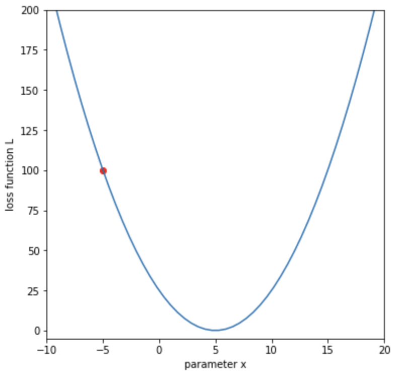
from matplotlib import animation, rc
from IPython.display import HTML

# 学習率(lr = learning rate)
lr = 0.2

# 摩擦や空気抵抗を考慮
momentum = 0.8

# Momentumオブジェクトの宣言
m = Momentum(lr,momentum)

# 更新回数
num_iterations = 50

# 初期値をコピー
x = x_initial

# 描画
fig = plt.figure(figsize=(6,6))
plt.plot(x_line, L_line)
images = []

for n in range(num_iterations):
    # 損失値を計算
    L = loss_function(x, a)
    # 勾配を計算
    grad = calc_gradient(x, a)

    print("%d-th iteration, x=%.3f, loss: %.3f, grad: %.3f" % (n, x, L, grad))

    # 更新前の状態を描画
    tangent = grad * (x_line - x) + L
    img = plt.plot(x_line, tangent, color='r')
    img.append(plt.scatter(x, L, color='r'))
    img.append(plt.text(-8, 180, 'iteration: '+str(n), size='x-large'))
    images.append(img)

    # 更新
    x = m.update(grad,x)

plt.xlim([-10, 20])
plt.ylim([-5, 200])
plt.xlabel('parameter x')
plt.ylabel('loss function L')

# アニメーション作成
anim = animation.ArtistAnimation(fig, images, interval=100)

# Google Colaboratoryの場合必要
rc('animation', html='jshtml')
plt.close()
display(anim)
ボールが転がるように、損失関数が最小化していくことがわかります。
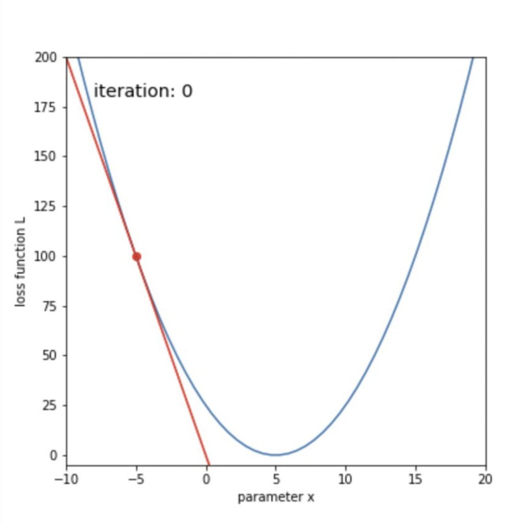
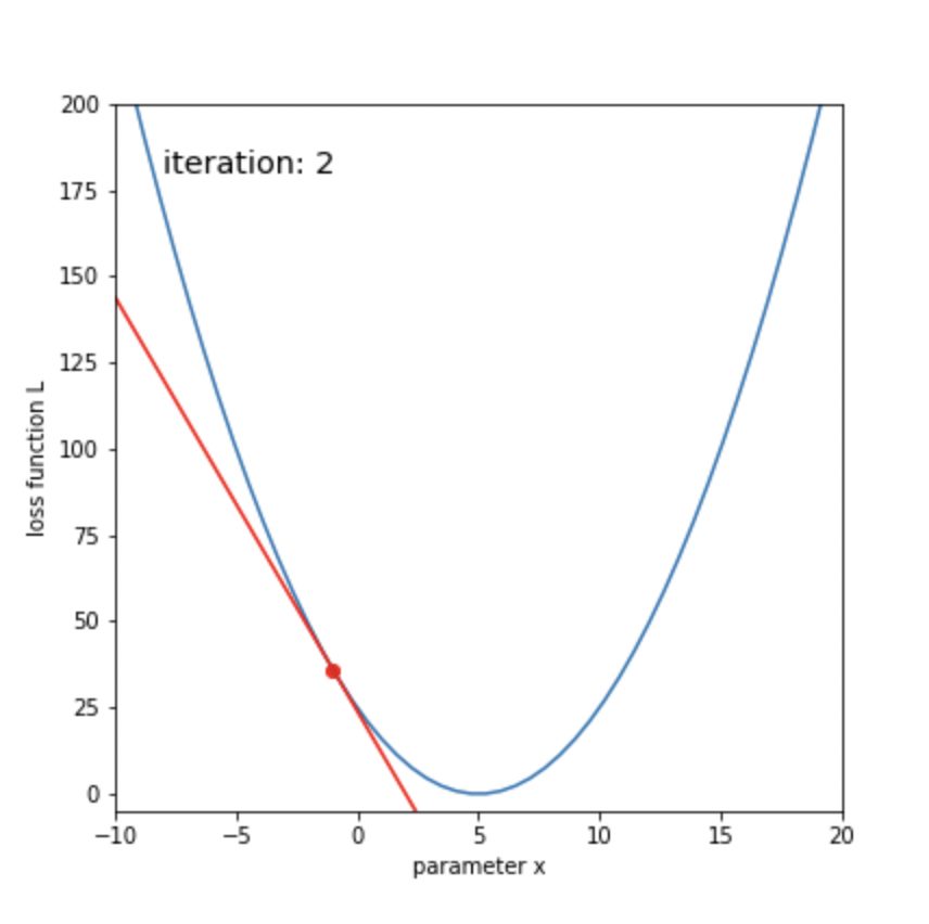
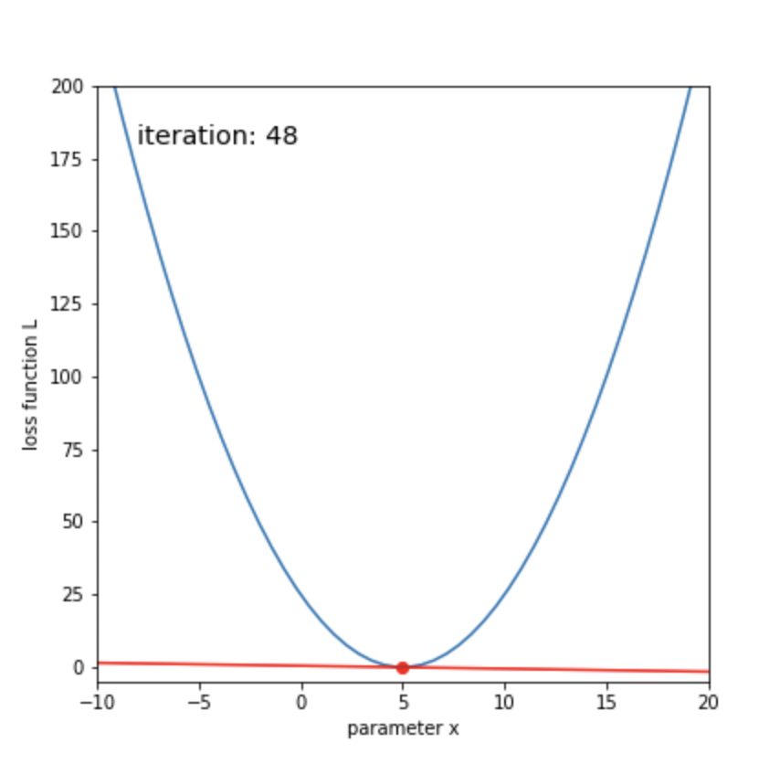
50回ほどの更新で、xが目標の5に辿り着いたことがわかります。
まとめ
Momentum法とは、勾配方向に速度を取り入れたもので、ボールが転がるようなイメージ
\(v_{next} = αv_{initial} – η\frac{∂L}{∂x}\)
\(x_{next} = x_{initial} + v_{next}\)
αとηはハイパーパラメータ
今回はニューラルネットワークのMomentum法についてまとめました。
機械学習、ディープラーニングを学びたい方におすすめの入門書籍です。
ディープラーニングの理論が分かりやすくまとめられていて、力を身につけたい方におすすめです。
最後まで読んでいただきありがとうございました。
他にもいろんな記事があるにゃ。

コメント